How it Works

How led_blink_with_plot Works

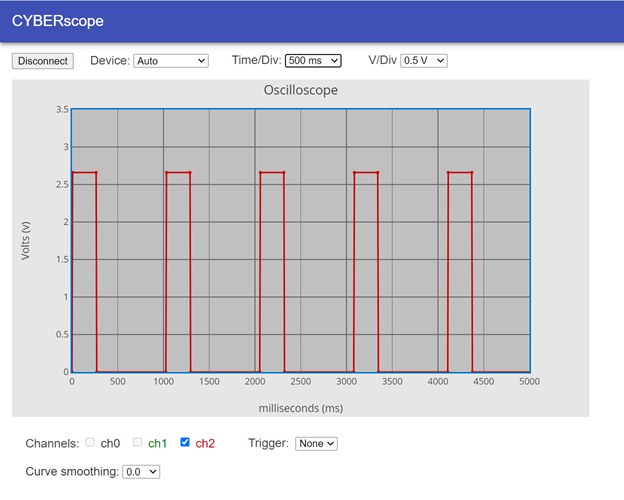
An oscilloscope plot graphs voltage over time.  Since your script turns the light on for 500 ms, then off for 500 ms, the plot shows the voltage repeatedly stays at 2.65 V for about half a second and then at 0 V for half a second.

As you can see the script timing is not precise.  It spends more than more than 500 ms high and low.  The reason for this is because it takes the micro:bit time to execute each statement, and it also takes time for it to send that data to the CYBERscope.  

When you adjusted the Time/Div from 1000 ms to 500 ms, you changed the x-axis increments from 1000 ms to 500 ms.  The total amount of time it graphed dropped from 10,000 ms to 5000 ms.

This script also started as led_blink from Connect and Blink a Light.  Again, the multimeter module is imported for sending data to the CYBERscope.  The plot data is sent to the CYBERscope with plot(volts(pin2),”y2″).  The plot function sends data to the CYBERscope formatted so that it can be plotted in the oscilloscope display.  The value it sends is volts(pin2), which measures the voltage with the P2 pin (through the red alligator clip lead).  The “y2” text string is forwarded to the CYBERscope, which results in the data being plotted on its red channel 2 (ch2) trace.

# led_blink_with_plot                     # <-- changed

from microbit import *
from multimeter import *                  # <-- added

while True:

    pin13.write_digital(1)
    sleep(1)                              # <-- added
    plot(volts(pin2), "y2")               # <-- added
    sleep(499)                            # <-- changed
    plot(volts(pin2), "y2")               # <-- added

    pin13.write_digital(0)
    sleep(1)                              # <-- added
    plot(volts(pin2), "y2")               # <-- added
    sleep(499)                            # <-- changed
    plot(volts(pin2), "y2")

The measurements have to be plotted before and after each pin13.write_digital call.  Normal oscilloscopes send many data points; whereas, this script sends just the points before and after each signal level change.  The sleep(1) is added between each pin13.write_digital call to give the voltage enough time to rise to its final value.

If you are curious why the sleep wasn’t needed for the voltmeter but is needed here, it’s because voltmeter() measurements are actually the average of ten measurements, taken every 10 ms.  In contrast volts() is a single measurement.

Try This: 25% Duty Cycle

In the main activity, you experimented with a 50% duty cycle signal.  The high and low times were equal, and the plot showed that.  Here, you will change it to a 25% duty cycle and observe the differences in the CYBERscope.

• In the script, try changing the first sleep(500) to sleep(250) and the second sleep(500) to sleep(750).
• Click the CYBERscope’s Disconnect button.
• In the micro:bit Python Editor, Send to micro:bit.
• Click the three vertical dots  ⋮  by the Send to micro:bit button, and select Disconnect.
• Back in the CYBERscope, click the Connect button.
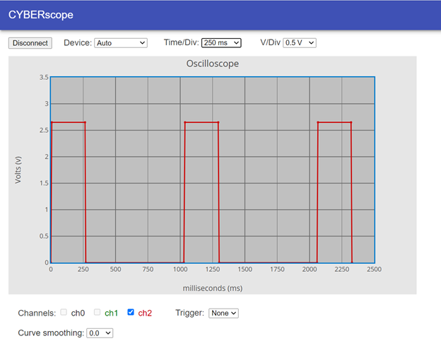
• Verify that the plot now resembles the image below.  See how the plot shows the signal as high (around 2.65 V) for about 250 ms and low (0 V) for about 750 ms?

• Try taking a closer look at the signal timing by changing the Time/Div dropdown to 250 ms.  
• Verify that the result should resemble the image below. Can you see what changed?