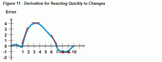
Here's a situation that neither proportional nor integral control really deal with. It's rapid changes to the system that come from an external source. Keeping the system steady when outside influences are making it change abruptly is the job of derivative control. In calculus, derivative is an operation that measures the rate of change of a curve, such as the error curve shown in Figure 11. By taking action based on the rate the error is changing, the output drive can respond rapidly to disturbances to the system.

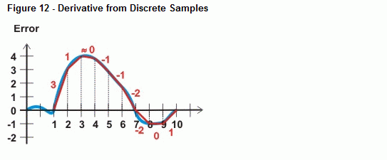
Like the samples in Figure 11, calculus can be used to examine any point on the curve and give you an exact slope. Circuits that involve operational amplifiers do these continuous calculations for continuous time control systems. When a signal is digitally sampled periodically, the derivative can be an algebraic slope calculation. The BASIC Stamp can then take the difference between two sampled points on a curve, and divide by the distance (time) between those two points.

In the case of the error vs. time graph, derivative would be the change in error divided by the change in time. That's ∆e/∆t. As with integration, numerical differentiation (calculating the derivative) can be simplified for control purposes by always considering the time between samples to be a value of 1. Then, numerical differentiation can be accomplished by subtracting the value of the previous error measurement from the current error measurement. In other words, derivative control can be accomplished with simple subtraction:
' Calculate derivative term.
error(Delta) = error(Current) - error(Previous)
d = Kd * error(delta)
Although ∆t might be a small or a large value, so long as it's always the same interval, the derivative constant, Kd can be scaled to compensate for the fact that we made ∆t equal to 1. Keep in mind that the rate that the errors are sampled also has to be faster than the error signal's tendency to change.
The job of derivative control is to react to changes in the system. For example, a constant error of -3 will be dealt with by proportional and integral control, but derivative won't touch it. Why? Because derivative only reacts to changes. With a series of errors of the same value, there's no change. However, any kind of change, such as the error going from -3 to 4, will cause derivative control to resist. Let's try an example program and observe how this works.
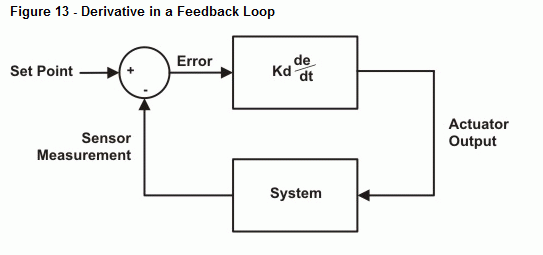
Figure 13 shows a block diagram for the derivative control loop the next example program will emulate. As with the other examples, Kd will be 10. This program will measure the rate of change of the error measurement (de/dt) and multiply by Kp = 10. This result will go to your Debug Terminal (actuator output).

Example Program - DerivativeAlgorithm.bs2
Try entering a series of sensor inputs that don't change, like 3 3 3 3 3 3 3 -4. Derivative will resist the first 3 because that's a change from 0 to 3, but all the rest of the threes will result in no correction from the derivative calculation. Then, with the big change from 3 to -4, the derivative will drive hard to correct this abrupt change.
- Enter, save, and run DerivativeAlgorithm.bs2.
- Try 3 3 3 3 3 3 3 -4. Verify that derivative resisted the first 3 but made no attempt to correct the others.
- Also verify that the the big change from 3 to -4 resulted in a large output to correct the change in error.
' DerivativeAlgorithm.bs2
' Demonstrates how derivative influences error correction
' in a feedback loop.

' {$STAMP BS2}
' {$PBASIC 2.5}

SetPoint       CON     0                     ' Set point
Kd             CON     10                    ' Derivative constant

Current        CON     0                     ' Current error
Previous       CON     2                     ' Previous error
Delta          CON     3                     ' Accumulated error

sensorInput    VAR     Word                  ' Input
error          VAR     Word(4)               ' Different types of errors
d              VAR     Word                  ' Derivative term
drive          VAR     Word                  ' Output

DO

  DEBUG "Enter sensor input value: "
  DEBUGIN SDEC sensorInput

  ' Calculate error.
  error(Current) = SetPoint - sensorInput

  ' Calculate derivative term.
  error(Delta) = error(Current) - error(Previous)
  d = Kd * error(delta)

  ' Calculate output.
  drive = d

  ' Display values.
  DEBUG CR, CR, "ERROR", CR,
        SDEC ? SetPoint, SDEC ? sensorInput, SDEC ? error(Current), CR,
        "DERIVATIVE", CR,
        SDEC ? Kd, SDEC ? error(Delta), SDEC ? d, CR,
        "OUTPUT", CR,
        SDEC ? d, SDEC ? drive, CR, CR

  ' Save current error to previous error before next iteration.
  error(Previous) = error(Current)

LOOP
How DerivativeAlgorithm.bs2 Works
The error array variable now has four elements. Element 0 is still the current error, element 1 is the accumulator, which is unused at present since there are not integral calculations in this program. Element 2 is used to store the previous error measurement, and element 3 is used to store the difference between the previous and current measurements. The constant for element 2 is Previous, and the constant for element 3 is Delta. That makes the derivative calculation much easier to read.
' Calculate derivative term.
error(Delta) = error(Current) - error(Previous)
d = Kd * error(delta)
At the end of each pass through the loop, the current measurement has to be saved as the previous measurement. There will be a new error(current) the next time through the loop, and a new error(delta) will be made with the updated error(Previous) value.
' Save current error to previous error before next iteration.
error(Previous) = error(Current)
Your Turn - Increasing the Reaction to Abrupt Changes
- Try changing the derivative constant (Kd) from 10 to 20.· It should react twice as strongly as before to abrupt changes in the error.
