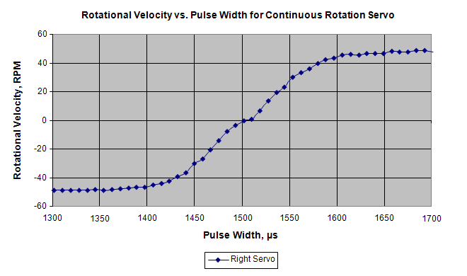
This graph shows pulse time vs. servo speed. The graph’s horizontal axis shows the pulse width in microseconds (µs), and the vertical axis shows the servo’s response in RPM. Clockwise rotation is shown as negative, and counterclockwise is positive. This particular servo’s graph, which can also be called a transfer curve, ranges from about -48 to +48 RPM over the range of test pulse widths from 1300 to 1700 µs. A transfer curve graph of your servos would be similar.
Three Reasons Why the Transfer Curve Graph is Useful
- You can get a good idea of what to expect from your servo for a certain pulse width. Follow the vertical line up from 1500 to where the graph crosses it, then follow the horizontal line over and you’ll see that there is zero rotation for 1500 µs pulses. We already knew servoLeft.writeMicroseconds(1500) stops a servo, but try some other values.
- Compare servo speeds for 1300 and 1350 µs pulses. Does it really make any difference?
- What speed would you expect from your servos with 1550 µs pulses? How about 1525 µs pulses?
- Speed doesn’t change much between 1300 and 1400 µs pulses. So, 1300 µs pulses for full speed clockwise is overkill; the same applies to 1600 vs. 1700 µs pulses for counterclockwise rotation. These overkill speed settings are useful because they are more likely to result in closely matched speeds than picking two values in the 1400 to 1600 µs range.
- Between 1400 and 1600 µs, speed control is more or less linear. In this range, a certain change in pulse width will result in a corresponding change in speed. Use pulses in this range to control your servo speeds.